Performance Comparison of Auto-Regressive Moving Average (ARIMA) and Artificial Neural Networks (ANN) in Ginger Price and Output Forecasting in Nigeria (2021–2025)

Fidelis Tanko; Faith Debaniyu Ibrahim; Ezekiel Salawu Yisa; Alaba Olanike Ojo

doi:doi:10.11648/j.ijdsa.20261204.12

Research Article |

| Peer-Reviewed

Performance Comparison of Auto-Regressive Moving Average (ARIMA) and Artificial Neural Networks (ANN) in Ginger Price and Output Forecasting in Nigeria (2021–2025)

Fidelis Tanko^*

, Faith Debaniyu Ibrahim

, Ezekiel Salawu Yisa

, Alaba Olanike Ojo

Published in International Journal of Data Science and Analysis (Volume 12, Issue 4)

Received: 15 March 2026 Accepted: 25 March 2026 Published: 27 July 2026

Views: Downloads:

Download PDF

Share This Article

Twitter
Linked In
Facebook

Abstract

This study analyzed and forecasted ginger output and price trends in Nigeria using Autoregressive Integrated Moving Average (ARIMA) and Artificial Neural Network (ANN) models. Secondary data on ginger production and price covering the period 1990–2020 were obtained from the Food and Agriculture Organization (FAO) and the National Agricultural Extension and Research Liaison Services (NAERLS). The data were analyzed to generate forecasts for the period 2021–2025. Stationarity of the time series was tested using the Augmented Dickey–Fuller (ADF) and Phillips–Perron tests, which indicated that both output and price series became stationary after first differencing. Model identification was conducted using the Autocorrelation Function (ACF) and Partial Autocorrelation Function (PACF). The most suitable ARIMA models selected were ARIMA (6,1,5) for ginger output and ARIMA (9,1,5) for ginger price based on model diagnostics such as AIC, SBIC, R-squared, and volatility measures. For ANN forecasting, optimal network structures identified were 1–10–1 for ginger output and 1–16–1 for ginger price, which produced the lowest network errors. Forecast evaluation showed that both ARIMA and ANN models produced relatively low forecast errors, indicating good predictive performance. However, the ANN model demonstrated slightly higher forecasting accuracy than the ARIMA model for both ginger output and price. Forecast results indicate a steady increase in ginger production from about 608,080 metric tonnes in 2021 to 719,968 metric tonnes by 2025, while prices are projected to rise gradually over the same period. The findings suggest growing demand for ginger at local and international market.

Published in	International Journal of Data Science and Analysis (Volume 12, Issue 4)
DOI	10.11648/j.ijdsa.20261204.12
Page(s)	69-84
Creative Commons	This is an Open Access article, distributed under the terms of the Creative Commons Attribution 4.0 International License (http://creativecommons.org/licenses/by/4.0/), which permits unrestricted use, distribution and reproduction in any medium or format, provided the original work is properly cited.
Copyright	Copyright © The Author(s), 2026. Published by Science Publishing Group

Keywords

Ginger, Price, Output, Forecasting, ARIMA, ANN

1. Introduction

Agriculture remains a key sector of Nigeria's economy, significantly contributing to job creation, food security, and foreign exchange earnings. Among the various agricultural products, ginger (Zingiber officinale) stands out due to its high domestic demand and strong export market. Nigeria is one of the world’s leading ginger producers and the largest in Africa, with production mainly concentrated in Kaduna, Plateau, Nasarawa, and Gombe states

[3]

. Ginger valued globally for its distinctive aroma, high oil content, and pungency, ginger is a crucial commodity in the international spice trade. Consequently, ginger farming is essential for supporting rural livelihoods, fostering agribusiness growth, and enhancing export diversification in Nigeria. The Nigerian ginger industry has experienced significant shocks in recent years, especially between 2021 and 2025, including disease outbreaks and supply chain disruptions that affected production levels and market supply. Such instability often leads to unpredictable price movements, which can negatively affect farmers' income, traders' profitability, and government planning in the agricultural sector. Despite its economic importance, the ginger sector in Nigeria has been characterized by considerable fluctuations in both output and market prices

[16]

Effective decision-making and policy planning so depend on accurate forecasting of agricultural commodity prices and output. Precise forecasts facilitate the planning of agricultural operations by farmers, allow traders to control market risks, and help policymakers create suitable measures to stabilise markets. Agricultural market patterns have long been predicted using time series forecasting techniques. Because it can identify linear trends and temporal links in historical data, the Auto-Regressive Integrated Moving Average (ARIMA) model is one of the most used classical statistical models. Numerous agricultural and economic time series have been successfully modelled and forecasted using ARIMA models.

However, the forecasting ability of conventional linear models may be limited by the nonlinear patterns, structural changes, and intricate interactions among variables that are frequently present in agricultural pricing and production data. In recent years, machine learning techniques like Artificial Neural Networks (ANN) have drawn more attention in response to these constraints. ANN models are computer systems that can learn intricate nonlinear correlations from data and are modelled after the structure of the human brain

[15]

. ANN models have been extensively used in financial, agricultural, and economic forecasting due to its flexibility and capacity for adaptive learning.

The usefulness of statistical and machine learning models in predicting agricultural commodity prices and production levels has been the subject of numerous research. ANN models are frequently acknowledged for their capacity to identify nonlinear patterns and enhance prediction accuracy, whereas ARIMA models are renowned for their solid theoretical underpinnings and interpretability

[7]

. However, the exact commodity under consideration, the forecasting horizon, and the type of data can all affect how well these models perform in comparison.

Given the increasing value of ginger in Nigeria's agricultural economy and the rising price and output volatility, it is necessary to assess suitable forecasting methods that can produce accurate forecasts. To ascertain whether method provides superior prediction performance for the dynamics of the Nigerian ginger market, a comparative study of forecasting models is necessary. Thus, the purpose of this study is to evaluate how well Artificial Neural Networks (ANN) and the Auto-Regressive Integrated Moving Average (ARIMA) model anticipate the price and output of ginger in Nigeria between 2021 and 2025.

It is anticipated that the results of this study would add to the body of knowledge on agricultural forecasting and offer helpful information to researchers, farmers, traders, and policymakers who want to enhance market forecasting and planning in the Nigerian ginger industry.

2. Research Methodology

2.1. Study Area

This study was conducted in Nigeria. Nigeria is located in West Africa on the Gulf of Guinea and is one of the largest countries in Africa, occupying a geographical area of about 923,770 square kilometers with an estimated population of 223,804,632 and a population growth rate of 2.4%

[18]

. It lies along latitudes 9° 04' 39.90" N and longitudes 8° 40' 38.84" E. It is bounded by the Atlantic Ocean to the south and by the Sahelian countries of Niger and Chad to the North. Nigeria operate operates Federal system of government with 36 States and Federal Capital Territory and 774 Local Government Areas (LGAs). Nigeria, by virtue of its location, enjoys a warm tropical climate with relatively high temperatures throughout the year and two seasons: the rainy or wet season that lasts from mid-March to November in the south and from May to October in the north, and the dry season that occupies the rest of the year. Secondary data, such as price and output of ginger, were sourced from the Food and Agriculture Organization's (FAO)

[6]

website and the National Agricultural Extension Research Liaison Services (NAERLS)

[10]

, from 1990–2020. The data collected were analyzed using ARIMA and ANN methodologies to forecast both output and price from 2021 to 2025, respectively.

2.2. Model Specification

ARIMA has three parts like Auto Regressive (AR), Integrated (I) and Moving Average (MA) (p,d,q.).

The general model specification is expressed as follows, consistent with the approach described by

[8, 17]

∆^{d} {PG}_{t} = δ + θ_{1} ∆^{d} {PG}_{t - 1} + θ_{2} ∆^{d} {PG}_{t - 2} + \dots \dots \dots θ_{p} {PG}_{t - p} + e_{t - 1} \propto_{2} e_{t - 2} \propto_{\infty} e_{t - 2}

(1)

∆^{d} Q_{t} = δ + θ_{1} ∆^{d} Q_{t - 1} + θ_{2} ∆^{d} Q_{t - 2} + \dots \dots \dots θ_{p} Q_{t - p} + e_{t - 1} \propto_{2} e_{t - 2} \propto_{\infty}

(2)

Where

∆^{d}

= differencing of order d, i.e.

∆ {PG}_{t} = y_{t} y_{t - 1} ∆^{2} {PG}_{t} = ∆ {PG}_{t} - ∆_{t - 1}

{PG}_{t}

= Price of ginger at year t,

{PG}_{t - 1} \dots \dots {PG}_{t - p} =

Previous observations (lags) of actual prices of ginger.

{\begin{matrix} δ \end{matrix}}_{1} = Constant

Q_{t - 1} \dots Q_{t - p}

= Previous observations (lags) of actual output of ginger

θ_{1}, θ_{2} \dots θ_{p}

= Coefficients of the lagged prices and output for the year under study (2021-2025) similar to regression coefficient of the Auto Regression process (AR) of order “p” and is written as:

{PG}_{t}

δ + θ_{1} {PG}_{t - 1} + θ_{2} {PG}_{t - 2} + \dots θ_{p} {PG}_{t - p} + e_{i}

(3)

Q_{t}

δ + θ_{1} Q_{t - 1} + θ_{2} Q_{t - 2} + \dots θ_{p} Q_{t - p} + e_{i}

(4)

Where;

{PG}_{t}

= Forecast prices (2021-2025).

{PG}_{t - 1} = lagged prices

Q_{t} =

Forecast output (2021-2025)

δ = costant, e_{t}

is a forecast error.

e_{t - 1,} \dots \dots e_{t - 2,} e_{t - p}

= Previous forecast error of prices and output

\propto_{1} - \propto_{p}

= Moving Average (MA) coefficients that needs to be estimated from the year 2021-2025.

ANN were used to obtain a robust and efficient forecasting. The time-series data were decomposed into positive and negative nonlinear components using the partial sum decomposition approach proposed by

[11, 13, 14]

Y_{t} = L_{t} + N_{t}

(5)

Where;

Y_t= Observed time series data.

L_t = Linear auto-regressive component.

N_t = Non-linear component.

This study employed a three-layer (one hidden layer) multilayer perceptron model trained with back-propagation algorithm. The ANN model used for the nonlinear data is represented as follows:

y_{t} = w_{0} + q \sum j = 1 w_{j} . g (w_{0 j} + p \sum i = i = {1 w}_{ij .} y_{t - 1)} + ε_{t}

(6)

Where,

𝑤_𝑖𝑗 (𝑖 = 0, 1, 2... 𝑝, 𝑗 = 1, 2... 𝑞) and 𝑤_𝑗 (𝑗 = 0, 1, 2... 𝑞) are the connection weights, 𝑝 is the number of input nodes, and 𝑞 is the number hidden nodes. Each grouped into two as inputs for day 𝑖-1 and day 𝑖-2, were supplied into the model. These variables are the opening price (𝑂_𝑖-1, 𝑂𝑖-2), annual high price or quantity (𝐻_𝑖-1, 𝐻_𝑖-2), annually low price or quantity, (𝐿𝑖-1, 𝐿_𝑖-2), annual closing price and output (𝐶_𝑖-1, 𝐶_𝑖-2), and trading volume (𝑉_𝑖-1, 𝑉_𝑖-2).

The creation of the ANN predictive model with Zaitun Time series involves the followings:

Creating the network topology. This involves the selection of the number of input neurons, the number of hidden layers, the number of hidden neurons in the hidden layer, and the number of output neurons. (in this case 1 input layer, 10 hiden layer, 1 output layer for output of ginger. While, 1 input layer, 16 hiden layer, 1 ouput layer for price of ginger).

Training the network. This involves selecting the network type/training algorithm, in our case feed forward back-propagation algorithm, inputting the training and target data, selecting the training function, selecting the adaptation learning function, selecting the performance function, and selecting the transfer function. The training parameters were set as follows: learning rate 0.05, momentum term 0.5, and epoch size 12000, 5000 respectively. Finally, the network was tested with the data set to estimate its generalization ability. To determine the best performing model, simulation experiment was run on different ANN model configurations. Both training and testing data were carefully selected. However, the training was not done with test data. The model was trained with different epochs, respectively, while the mean squared error (MSE) for each training session of the different network structure was usually noted. The network structure that returns the smallest MSE in each of the models is mainly adjudged the best model that can give the best accurate prediction.

3. Results and Discussion

3.1. Ginger Forecasting Using the ARIMA Model

3.2. Unit Root Test of the ARIMA Model

The result of the unit root test is shown in Table 1. The application of most time series models requires data to be stationary

[1]

. The ADF and the Philip-Perron test were applied to test the stationarity of all the data sets considered in this study. It was observed that the output and price of ginger were not stationary at this level (p-values > 0.05). However, the data sets were stationary after the first difference (p-values < 0.05). Thus, it was confirmed that the first differences for all series were perfect for modeling and forecasting.

Table 1. Estimate of unit root of the ARIMA.

Variables	Order	Exogenous	ADF test (P-value)	Critical value at 5%	Phillip-Perron test (P-value)	Critical value at 5%
ΔQT_t	1 (1)	Constant Constant and Trend	-5.3206 (0.0002)	-2.9678	-5.6299 (0.0001)	-2.9678
ΔQT_t	1 (1)	Constant Constant and Trend	-5.8259 (0.0003)	-3.5742	-5.8776 (0.0002)	-3.5742
ΔPG_t	1 (1)	Constant Constant and Trend	-5.2619 (0.0002)	-2.9719	-7.6717 (0.0000)	-2.9678
ΔPG_t	1 (1)	Constant Constant and Trend	-5.2186 (0.0012)	-3.5806	-9.2605 (0.0000)	-3.5742

Source: Analysed result from time series data 1990-2020 using EVIEWS 10

3.3. Identification of the ARIMA Models

Building an ARIMA model for any given time series involves the following four steps: identification of the model, estimation of parameters, diagnostic checking, and forecasting (Box-Jenkins, 1976). The first, which is otherwise imperative, is to verify if the mean, variance, and autocorrelation of the time series are consistent throughout the established interval. Therefore, two-time-series plots, the auto-correlation function (ACF), and the partial auto-correlation function (PACF) graphs were generated to test the seasonality and stationarity. ACF is a statistical metric that determines whether the prior values are related to the latest values, while PACF is the value of the correlation coefficient between its time lag and the variable. Both are imperative in detecting misspecification: the model performance being measured by Akaike information criteria expression and the Bayesian Information Criterion of Schwarz (BIC).

The auto-correlation function (ACF) and partial auto-correlation function (PACF) were used as tools for identifying the parameters of the model. The ACF and PACF at first difference for both ginger output and price are presented in Tables 2 and 3, respectively. In the observed structure of the production series for ginger output in Tables 2 and 3, both the ACF and the PACF have a significant spike at lag 5, and only the PACF has significant spikes at lag 6, indicating ARIMA models of ARIMA (5, 1, 5) and ARIMA (6, 1, 5). A diagnostic check on the selected model does not show any significant spike on the correlogram Q-statistics, and all the series are not significant as captured in the correlogram squared residuals test statistics. In the observed structure of the price of ginger series in Table 3, only the ACF and the PACF have a significant spike at lags 5 and 4, respectively, giving rise to ARIMA (4, 5). The correlogram Q-statistics test shows a significant spike of the PACF at lag 9, while all the series are not significant as captured in the correlogram squared residuals test statistics. Since there was a significant spike in the correlogram Q-statistics of the PACF, ARIMA (9,1,5) was also selected as a model.

Table 2. Correlogram of the output of ginger (Q_t) for model Identification at 1 (1).

Autocorrelation	Partial Correlation	No.	AC	PAC	-Stat	Prob
**\|. \|	**\|. \|	1	-0.278	-0.278	2.9393	0.086
. \|. \|	.*\|. \|	2	0.001	-0.083	2.9393	0.230
. \|** \|	. \|** \|	3	0.266	0.265	5.7923	0.122
.*\|. \|	. \|. \|	4	-0.175	-0.032	7.0659	0.132
. \|*** \|	. \|*** \|	5	0.359	0.357	12.628	0.027
**\|. \|	**\|. \|	6	-0.301	-0.260	16.662	0.011
. \|. \|	.*\|. \|	7	-0.037	-0.123	16.724	0.019
. \|*. \|	.*\|. \|	8	0.113	-0.174	17.339	0.027
.*\|. \|	. \|*. \|	9	-0.129	0.089	18.175	0.033
.*\|. \|	**\|. \|	10	-0.098	-0.291	18.669	0.045
.*\|. \|	. \|. \|	11	-0.132	-0.018	19.612	0.051
. \|*. \|	. \|. \|	12	0.088	-0.003	20.047	0.066
.*\|. \|	. \|. \|	13	-0.090	0.028	20.524	0.083
.*\|. \|	.*\|. \|	14	-0.087	-0.111	20.987	0.102
. \|. \|	. \|. \|	15	-0.022	0.029	21.018	0.136
. \|. \|	.*\|. \|	16	-0.021	-0.085	21.048	0.177

Source: Analysed result from time series data 1990-2020 using EVIEWS 10

Table 3. Correlogram of the price of ginger (PG_t) for model Identification at 1 (1).

Autocorrelation	Partial Correlation	No.	AC	PAC	Q-Stat	Prob
**\|. \|	**\|. \|	1	-0.246	-0.246	2.3025	0.129
.*\|. \|	**\|. \|	2	-0.187	-0.264	3.6797	0.159
. \|. \|	.*\|. \|	3	0.045	-0.090	3.7604	0.289
**\|. \|	***\|. \|	4	-0.241	-0.350	6.1957	0.185
. \|*** \|	. \|** \|	5	0.394	0.261	12.911	0.024
. \|. \|	. \|. \|	6	-0.041	0.010	12.985	0.043
.*\|. \|	. \|. \|	7	-0.148	0.017	13.995	0.051
. \|. \|	.*\|. \|	8	0.033	-0.068	14.047	0.081
**\|. \|	**\|. \|	9	-0.263	-0.221	17.495	0.042
. \|*. \|	**\|. \|	10	0.108	-0.208	18.101	0.053
. \|. \|	**\|. \|	11	-0.002	-0.266	18.102	0.079
. \|*. \|	. \|*. \|	12	0.152	0.170	19.405	0.079
. \|. \|	. \|. \|	13	-0.005	-0.018	19.406	0.111
**\|. \|	. \|. \|	14	-0.244	-0.018	23.088	0.059
. \|*. \|	. \|. \|	15	0.112	0.000	23.905	0.067
. \|*. \|	. \|*. \|	16	0.114	0.176	24.797	0.073

Source: Analysed result from time series data 1990-2020 using EVIEWS 10

3.4. Output of the Identified ARIMA Models

Table 4 describes the output of the identified ARIMA (5,1,5); ARIMA (6,1,5) for the production series of ginger output (qt); ARIMA (4,1,5); and ARIMA (9,1,5) for the price of ginger (pg), as suggested by their respective ACF and PACF structures. Given the selection criteria set in the methodology, it could be observed that ARIMA (6,1,5) for ginger output and ARMA (9,1,5) for the price of ginger were preferred to others in each of the respective categories because of their high numbers of significant coefficients, lowest volatility of 4.41E+09 for ginger output and 11052.42 for the price of ginger, highest R-Squared values of 0.316503 and 0.243612 in each of the categories, and the lowest AIC and SBIC of 25.33075 and 25.50850 for ginger output, respectively, and 12.42108 and 12.59884 for the price of ginger, respectively.. The selected model used for ARIMA forecasting was ARIMA (6,1,5) for ginger output and ARIMA (9,1,5) for the price of ginger. This result is similar to the findings of

[4]

, who reveal that ARIMA (1, 1, 1) and ARIMA (2, 1, 2) are the most suitable ARIMA for the cultivation area and production of maize in Nigeria. This further collaborated with

[12]

, who reported that ARIMA (1, 1, 1) is the most appropriate model to foretell future prices of groundnut in Odisha states of India in 2019.

Table 4. Output of the Identified ARIMA models.

Variables	Ginger Output (Qt)		Price of Ginger (PG)
Variables	ARIMA (5, 1, 5)	ARIMA (6, 1, 5)	ARIMA (4, 1, 5,)	ARIMA (9,1,5)
Sig. coefficients	1	2	2	2
Sigma² (volatility)	4.90E+09	4.41E+09	11861.74	11052.42
R-Squared	0.240572	0.316503	0.188225	0.243612
AIC	25.42599	25.33075	12.46898	12.42108
SBIC	25.60372	25.50850	12.64674	12.59884

Source: Analysed result from time series data 1990-2020 using EVIEWS 10

3.5. Diagnostics Testing of the Selected ARIMA Models

In order to be sure that the selected model has adequately captured all the inherent structure of differenced ginger output and price series, the correlogram Q-statistics and the correlogram squared residuals diagnostic procedures were employed in each of the models to determine the presence of significant spikes in the correlogram.

3.6. The Correlogram Q-Statistics

The Q-statistics for each of the ARIMA (6, 1, 5) and ARIMA (9,1,5) are presented in Tables 5 and 6. The result showed that the spikes remain within the 95% confidence interval for both ACF and PACF. This also confirms that all the structures within the equation were adequately accounted for by the models.

Table 5. Correlogram Q-statistics plot for ARIMA (6,1,5).

Autocorrelation	Partial Correlation	No.	AC	PAC	Q-Stat	Prob
.*\|. \|	.*\|. \|	1	-0.198	-0.198	1.4965	0.000
.*\|. \|	.*\|. \|	2	-0.077	-0.121	1.7295	0.000
. \|*** \|	. \|*** \|	3	0.424	0.404	9.0010	0.003
.*\|. \|	. \|. \|	4	-0.201	-0.063	10.695	0.005
. \|. \|	. \|*. \|	5	0.059	0.077	10.843	0.013
. \|. \|	**\|. \|	6	-0.053	-0.273	10.969	0.027
. \|. \|	. \|. \|	7	-0.053	0.035	11.097	0.049
. \|. \|	.*\|. \|	8	-0.003	-0.126	11.098	0.085
.*\|. \|	. \|*. \|	9	-0.072	0.099	11.353	0.124
. \|. \|	.*\|. \|	10	-0.026	-0.122	11.389	0.181
.*\|. \|	. \|. \|	11	-0.105	-0.056	11.985	0.214
. \|. \|	. \|. \|	12	0.060	-0.010	12.189	0.273
. \|. \|	. \|. \|	13	-0.037	0.025	12.270	0.344
.*\|. \|	. \|. \|	14	-0.082	-0.036	12.686	0.392
. \|. \|	.*\|. \|	15	-0.008	-0.129	12.690	0.472
. \|. \|	. \|. \|	16	-0.046	-0.061	12.833	0.540

Source: Analysed result from time series data 1990-2020 using EVIEWS 10

Table 6. Correlogram Q-statistics plot for ARIMA (9,1,5).

Autocorrelation	Partial Correlation	No.	AC	PAC	Q-Stat
. \|***** \|	. \|***** \|	1	0.711	0.711	19.737
. \|**** \|	. \|*. \|	2	0.553	0.097	32.042
. \|*** \|	. \|. \|	3	0.441	0.035	40.109
. \|** \|	. \|. \|	4	0.336	-0.024	44.938
. \|*** \|	. \|** \|	5	0.367	0.221	50.897
. \|*. \|	***\|. \|	6	0.163	-0.379	52.106
. \|. \|	.*\|. \|	7	0.005	-0.141	52.108
.*\|. \|	.*\|. \|	8	-0.125	-0.145	52.871
.*\|. \|	. \|. \|	9	-0.197	0.031	54.844
.*\|. \|	. \|*. \|	10	-0.106	0.156	55.432
.*\|. \|	. \|. \|	11	-0.119	0.061	56.214
.*\|. \|	. \|. \|	12	-0.117	0.055	56.990
.*\|. \|	. \|*. \|	13	-0.092	0.088	57.494
. \|. \|	. \|. \|	14	-0.065	0.031	57.759
. \|*. \|	. \|. \|	15	0.074	0.068	58.120
. \|*. \|	. \|. \|	16	0.132	-0.020	59.311

Source: Analysed result from time series data 1990-2020 using EVIEWS 10

3.7. Correlogram Squared Residuals Test

The residuals are not only random but are also independent of each other. The structures of each of the residual plots show no defined pattern as they randomly hover around zero. Tables 7 and 8 show the residual plots for ARIMA (6,1,5) and ARIMA (9,1,5). The result of the test shows that all the probability levels of the variables captured in the tables were not significant, hence the application of the selected model.

Table 7. Correlogram squared residuals plot for ARIMA (6,1,5).

Autocorrelation	Partial Correlation	No.	AC	PAC	Q-Stat	Prob
. \|** \|	. \|** \|	1	0.302	0.302	3.4809	0.062
. \|. \|	.*\|. \|	2	-0.023	-0.126	3.5020	0.174
. \|*. \|	. \|** \|	3	0.163	0.233	4.5725	0.206
. \|** \|	. \|** \|	4	0.324	0.223	8.9648	0.062
. \|*. \|	. \|. \|	5	0.120	-0.026	9.5848	0.088
. \|. \|	. \|. \|	6	-0.052	-0.063	9.7034	0.138
. \|. \|	. \|. \|	7	0.018	-0.020	9.7185	0.205
. \|*. \|	. \|. \|	8	0.109	0.013	10.288	0.245
. \|. \|	. \|. \|	9	-0.004	-0.058	10.289	0.328
.*\|. \|	. \|. \|	10	-0.070	-0.009	10.545	0.394
. \|. \|	. \|. \|	11	-0.057	-0.056	10.722	0.467
. \|. \|	. \|. \|	12	-0.028	-0.036	10.768	0.549
. \|. \|	. \|. \|	13	-0.064	-0.036	11.006	0.610
. \|. \|	. \|. \|	14	-0.064	0.007	11.255	0.666
. \|. \|	. \|. \|	15	-0.064	-0.027	11.523	0.715
.*\|. \|	. \|. \|	16	-0.066	-0.024	11.820	0.756

Source: Analysed result from time series data 1990-2020 using EVIEWS 10

Table 8. Correlogram squared residuals for ARIMA (9,1,5).

Autocorrelation	Partial Correlation	No.	AC	PAC	Q-Stat	Prob
**\|. \|	**\|. \|	1	-0.225	-0.225	1.9303	0.165
. \|. \|	. \|. \|	2	-0.010	-0.064	1.9343	0.380
. \|. \|	. \|. \|	3	-0.033	-0.053	1.9783	0.577
. \|*. \|	. \|*. \|	4	0.141	0.128	2.8145	0.589
. \|. \|	. \|*. \|	5	0.010	0.076	2.8192	0.728
.*\|. \|	.*\|. \|	6	-0.188	-0.172	4.3998	0.623
**\|. \|	***\|. \|	7	-0.238	-0.349	7.0214	0.427
. \|*. \|	. \|. \|	8	0.209	0.045	9.1205	0.332
.*\|. \|	.*\|. \|	9	-0.123	-0.089	9.8789	0.360
.*\|. \|	.*\|. \|	10	-0.076	-0.092	10.179	0.425
. \|. \|	. \|. \|	11	-0.021	0.022	10.201	0.512
. \|. \|	.*\|. \|	12	-0.002	-0.093	10.202	0.598
. \|*. \|	. \|*. \|	13	0.192	0.087	12.366	0.498
. \|. \|	. \|. \|	14	-0.054	0.024	12.543	0.563
.*\|. \|	. \|. \|	15	-0.066	-0.058	12.821	0.616
. \|. \|	.*\|. \|	16	0.013	-0.144	12.833	0.685

Source: Analysed result from time series data 1990-2020 using EVIEWS 10

3.8. Network Structure and Model Identification of the ANN Training

The results of the ANN model for the network training are indicated in Table 9. All trainings were subjected to a learning rate of 0.05 with a momentum of 0.5 for both output and the price of ginger. After several trainings with different network architectures based on our ANN algorithm, the network structure that returns the smallest network error (0.136530) was noted to give the best forecasting accuracy with the test data. It was observed that the network structure 1-10-1 (1 input layers, 10 hidden layers, and 1 output layer) with iteration 12,000 was the predictive model with the most accurate output prediction. However, in terms of the price of ginger, the smallest network error (1.571596) with the network structure 1-16-1 (1 input layers, 16 hidden layers, and 1 output layer) and iteration 5,000 was noted to give the best forecasting accuracy with the test data. The two-network structure for output and price of ginger was adopted for the ANN forecasting model.

Table 9. Network Training for Ginger Out and price.

Network	Ginger Output		Network	Price of Ginger
Structure	Iteration	Network Error	Structure	Iteration	Network Error
1-10-1	10,000	0.137391	1-5-1	2,000	1.599873
1-10-1	5,000	0.139902	1-5-1	5,000	1.577707
1-12-1	10,000	0.139263	1-10-1	2,000	1.602732
1-12-1	5,000	0.140860	1-10-1	5,000	1.578618
1-5-1	10,000	0.137685	1-12-1	2,000	1.607841
1-5-1	5,000	0.139743	1-12-1	5,000	1.578454
1-10-1	12,000	0.136530	1-16-1	2,000	1.617408
1-5-1	12,000	0.137861	1-16-1	5,000	1.571596
1-12-1	12,000	0.137471

Learning Rate = 0.05 Momentum = 0.5

Sources: Analysed Result from time series data 1990-2020 (Zaitun time series)

3.9. The Predictive Strength of the ARIMA and ANN Model for the Output of Ginger from 2000 - 2025

Table 10 shows the predicted values for ginger output. Since ARIMA (6, 1, 5) and ANN (1-10-1) with iteration 12,000 proved to be a good fit to the model (1990–2020), the models were deployed to predict the selected out of sample series from 2021 to 2025 at a 95% confidence interval. According to the results, both the ARIMA and ANN models used for the output of ginger have a low forecast error, but the ANN model has a lower forecasting error than the ARIMA model. Further results show that the forecasting accuracy level of the ANN model compared with that of the ARIMA model is not quite significant. It can be argued that both models achieved good forecast performance judging from the forecast errors of both models, which are quite low. However, the performance of the ANN model is better than that of the ARIMA model in terms of forecasting accuracy on many occasions from the test data for ginger output. This finding agrees with the work of

[5]

where a statistical test was carried out, and the result also showed that there is no significant difference between the actual and predicted values of the two models, as the values of ANN and ARIMA are 0.439 and 0.604, respectively. Notwithstanding, ANN was still better.

Table 10. Sample of Predicted result of ARIMA (6, 1, 5) and ANN (1-10-1) for ginger output.

Sample period	ARIMA (6,1,5) Predictions for Ginger Output			ANN (1-10-1) Predictions for Ginger Output
Sample period	Actual values	Predicted values	Forecast Error	Actual values	Predicted values	Forecast Error
2000	142000	150829.6	-0.062	142000	135749.13	0.044
2001	114000	179921.1	-0.578	114000	148625.4	-0.304
2002	105000	196209.3	-0.869	105000	122001.96	-0.162
2003	110000	236515.0	-1.150	110000	114314.36	-0.039
2004	117000	242435.5	-1.072	117000	118533.98	-0.013
2005	125000	273349.7	-1.188	125000	124657.25	0.003
2006	134000	296065.5	-1.209	134000	131967.67	0.015
2007	162390	315936.7	-0.946	162390	140595.13	0.134
2008	145070	340823.1	-1.349	145070	170633.94	-0.176
2009	168800	356301.5	-1.110	168800	151797.62	0.101
2010	172223	385249.1	-1.237	172223	178006.4	-0.034
2011	260179	404406.3	-0.554	260179	182030.86	0.300
2012	380000	426774.9	-0.123	380000	303399.51	0.202
2013	413382	450257.8	-0.089	413382	488128.95	-0.181
2014	496920	471776.2	0.051	496920	534252.94	-0.075
2015	604900	496979.8	0.178	604900	629758.01	-0.041
2016	774887	516907.4	0.333	774887	711548.28	0.082
2017	700000	540670.0	0.228	700000	774604.61	-0.107
2018	734634	563174.6	0.233	734634	754096.45	-0.026
2019	927041	585242.7	0.369	927041	764731.85	0.175
2020	734295	608080.4	0.172	734295	794717.14	-0.082

Sources: Analyses output from time series 1990-2020

Table 11 shows the predicted values for the price of ginger. Since ARIMA (9,1,5) and ANN (1-16-1) with iteration 5,000 proved to be a good fit to the model (1990–2020), the models were deployed to predict the selected out of sample series from 2020 to 2025 at a 95% confidence interval. According to the results, both the ARIMA and ANN models used for the price of ginger also have a low forecast error, but the ANN model has a lower forecast error than the ARIMA model.

Further result also shows that the forecasting accuracy level of the ANN model compared with that of the ARIMA model in terms of the price of ginger is not also quite significant. It can also be argued that both models achieved good forecast performance judging from the forecast error of both models which are quite low, however, the performance of ANN model is better than ARIMA model in terms of forecasting accuracy on many occasions from the test data for the price of ginger. This finding agrees with the work of

[2]

which shows that ANNs outperformed ARIMA in predicting stock price movement direction as the latter was able to detect hidden patterns in the data used.

Table 11. Sample of forecasted result of ARIMA (9, 5, 1) and ANN (1-16-1).

Sample period	ARIMA (9,1,5) forecast for price of Ginger			ANN (1-16-1) predictions for price of ginger
Sample period	Actual values	Predicted values	Forecast Error	Actual values	Predicted values	Forecast error
2000	450.000	528.8627	-0.17525044	450.000	581.0511	-0.29122
2001	450.000	550.2959	-0.22287978	450.000	529.1941	-0.17599
2002	654.000	532.9301	0.185122171	654.000	529.1941	0.190835
2003	654.000	613.1564	0.062451988	654.000	583.5722	0.107688
2004	662.970	674.5768	-0.01750728	662.970	583.5722	0.119761
2005	690.500	684.8638	0.008162491	690.500	582.3567	0.156616
2006	480.000	701.0446	-0.46050958	480.000	577.7639	-0.20367
2007	398.500	640.6039	-0.60753802	398.500	553.4593	-0.38886
2008	483.000	632.0302	-0.30855114	483.000	467.1586	0.032798
2009	524.700	652.6720	-0.24389556	524.700	555.4321	-0.05857
2010	610.000	662.5365	-0.08612541	610.000	575.5867	0.056415
2011	385.000	683.8351	-0.77619506	385.000	587.0315	-0.52476
2012	385.000	676.3734	-0.75681403	385.000	447.1841	-0.16152
2013	379.540	674.4538	-0.77702956	379.540	447.1841	-0.17823
2014	562.970	687.6032	-0.22138515	562.970	438.8096	0.220545
2015	676.330	699.0156	-0.03354221	676.330	584.5499	0.135703
2016	524.700	733.0082	-0.39700438	524.700	580.2807	-0.10593
2017	666.279	751.7158	-0.12822977	666.279	575.5867	0.136118
2018	683.640	761.8136	-0.11434907	683.640	581.8711	0.148863
2019	500.000	775.0874	-0.5501748	500.000	579.0206	-0.15804
2020	666.290	784.9916	-0.17815306	666.290	565.2031	0.151716

Sources: Analyses output from time series 1990-2020 using EVIEWS 10 and Zaitun time series

3.10. The Out of Sample Forecasting for ARIMA and ANN Model from 2021-2025

The result of the out-of-sample forecast of both the ARIMA and ANN models for ginger output and price is indicated in Table 12. According to the results of ARIMA (6, 1, 5), the forecast of ginger output shows a continued increase in ginger production on a yearly basis from 608080.4 MT in 2021 to 719967.6 MT in 2025. This is also applicable to the result of ANN (1-10-1) which also shows a continued increase in ginger output from 764790.0953 MT in 2021 to 774051.5505. However, the increment associated with the output of the ginger forecast from the ARIMA model was lower than the forecast from the ANN model.

The increase in the future of ginger supply as observed in Table 12 may have occurred because ginger rhizome is a highly sought-after commodity in Asia, Europe, and America; it is widely used in food seasonings; and the root crop is increasingly seeing local and global demands. Farmers have also taken it seriously to add value to their crop in order to unlock potential to earn substantial dollars for the country. Additionally, ginger farming has been introduced to other states, just as a few states cannot feed the whole world with ginger.

Likewise, in recent years, interest in ginger in any of its various forms has been increasing as it is seen as a preventive or therapeutic agent. As such, Nigeria’s production and sales will also be on the increase to meet both local and international demands. This coincided with the objectives and targets of the National Development Plan (NDP, 2021–2025). The broad objective of the agriculture plan is to increase the sector’s productivity to drive economic growth and meet domestic demand for food. This further stated that by 2025, Nigeria’s agricultural productivity is expected to increase as technology, innovation, and climate-smart practices are introduced to ensure the continuous availability of affordable and nutritious food.

The forecast for the price of ginger from ARIMA (9,1,5) shows an expected high but steady price increase from ₦803.3715 in 2021 to ₦851.404 in 2025 as compared with the ANN (1-16-1) with a slow but steady price increase from ₦581.1313 in 2021 to ₦585.4804 in 2025.. The price change as captured in the model was steady, therefore ginger farmers will find it easier to respond positively to a change in ginger output as a result of the changes in ginger price in the future. This is in line with the study of

[9]

, who opined that ginger farmers find it difficult to predict the price of ginger in a situation of price fluctuation and, as such, maintain an increase in production within some given period of time when the price change is steady.

Although the ginger market valuation is expected to reach USD 3.42 billion by 2023, at a CAGR of 6.6%, According to Expert Market Research, however, the global ginger market size attained a value of USD 5.78 billion in 2022, while the market is projected to grow further at a CAGR of 4.5% to reach a value of USD 7.53 billion within a forecast period of 2023–2028.. However, the study already reveals that the forecast error for both the ARIMA and ANN models is moderately low, as the predicted values are close to the actual values and move in the direction of the forecast values in many instances, thereby providing insight that the agriculture sector remains a critical lever for ensuring economic development and the wellbeing of Nigeria’s populace. With a focus on increasing sector productivity and value addition, Nigeria will transform agriculture into a more significant component of its concentric diversification agenda, resulting in inclusive growth and development.

Table 12. Out of Sample Forecast of the ARIMA and ANN Model from 2021 - 2025.

Year	ARIMA Forecast		Year	ANN Forecast
	Qt	Pg		Qt	Pg
2021	629474.5	803.3715	2021	764790.0953	581.1313
2022	652935.4	820.1181	2022	772122.3266	585.2562
2023	674894.0	832.4239	2023	773670.3426	585.4703
2024	697345.3	845.2415	2024	773987.1425	585.4799
2025	719967.6	851.4048	2025	774051.5505	585.4804

Sources: Analyses output from time series 1990-2020 using EVIEWS 10 and Zaitun time series)

3.11. The Forecasting Trend of the ARIMA and ANN Model for the Output of Ginger

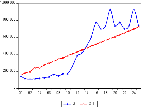
The ARIMA (6,1,5) and ANN (1-10-1) distributions of the historical series of the actual and forecasted ginger output indicators are shown in Figures 1 and 2. The forecast captured the period from 2000 to 2025. The result of the ARIMA (6,1,5) for ginger output shows the forecast graph in red and the actual output in blue. There was a wide deviation in the predictive power of the model from 2000 to 2012; the prediction from 2012 to 2014 was almost exact and became exact in 2015; there was a slight deviation in the forecasting strength of the model from 2015 to 2024 and became exact in 2025.

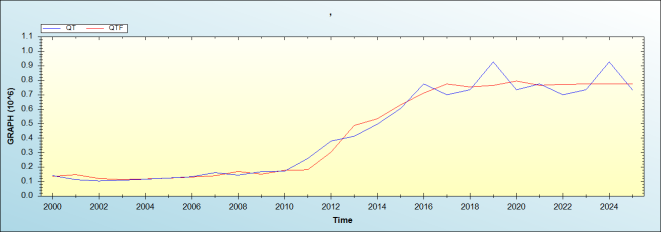
The result of the ANN (1-10-1) for the output of ginger also shows the forecast output graph in red and the actual output of ginger in blue. The forecasting power of the model indicates a closer range and similar predictions than the ARIMA model with the same and similar predictions of the actual ginger output flows from 2002 to 2010, with only a few cases, of close-range deviation. There was a close deviation in the predictive power of the model from 2010 to 2013, 2015, 2016, 2018, 2021, and 2023.

Download: Download full-size image

Figure 1. Fitted forecast of ARIMA (6,5,1).

Sources: Analyses output from time series 1990-2020 using EVIEWS 10 and Zaitun time series

Download: Download full-size image

Figure 2. Fitted Forecast of ANN (1-10-1).

3.12. The Forecasting Trend of the ARIMA and ANN Model for the Price of Ginger

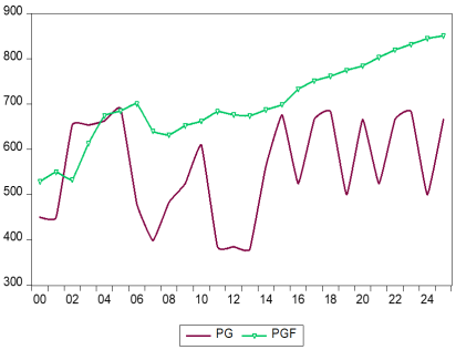
The ARIMA (9,1,5) and ANN (1-16-1) distributions of the historical series of the actual and forecasted ginger price indicators are shown in Figures 3 and 4. The forecast captured the period from 2000 to 2025. The result of the ARIMA (9,1,5) for the price of ginger shows the forecast graph in light green and the actual price of ginger in dark brown. The forecasting power of the model indicates the same and similar predictions of the actual price in 2002 and between 2004 and 2006. There was a wide deviation in the predictive power of the model from 2007 to 2015, 2017 to 2019, and between 2020 and 2025. The predictions for 2010, 2015, 2017, 2021, and 2022 were slightly off from the actual values.

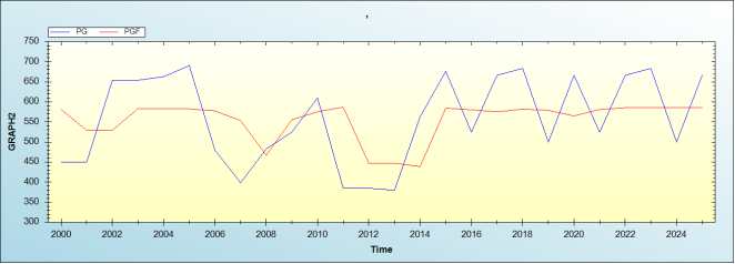
The result of the ANN (1-16-1) for the price of ginger also shows the forecast output graph in red and the actual output of ginger in blue. The forecasting power of the model indicates a closer range and similar predictions than the ARIMA model. There was a wide range deviation of the predictive power from the year 2000 and became exact mid-2001 and 2002; the deviation became wider between 2002 and 2005 and became exact mid-2005 and 2006. The trend continues from mid-2005 to 2007 and becomes exact in mid-2007 and in 2008.

A close deviation was observed between 2008 and 2009 becoming exact at 2010. Further result shows a wide range of deviation from 2010 to mid-2014, the deviation from the actual values follows a similar pattern, becoming exact at 2015, mid 2016, 2018, 2019, mid 2020, mid 2021, mid 2023 and 2024.

Download: Download full-size image

Figure 3. Fitted forecast for ARIMA (9,1,5).

Sources: Analyses output from time series 1990-2020 using EVIEWS 10 and Zaitun time series

Download: Download full-size image

Figure 4. Fitted forecast for ANN (1,16,1).

4. Conclusion

The study analyzed and forecasted ginger output and price in Nigeria using the Autoregressive Integrated Moving Average (ARIMA) model and Artificial Neural Network (ANN) based on time-series data from 1990–2020. The findings showed that the chosen ARIMA models ARIMA (6,1,5) for ginger production and ARIMA (9,1,5) for ginger price passed the necessary diagnostic tests and sufficiently reflected the data's structure following initial differencing. Both the ARIMA and ANN models' forecasting outputs demonstrated comparatively low prediction errors, suggesting that both models are trustworthy for predicting trends in agricultural commodities. Nonetheless, the ANN model showed somewhat higher prediction accuracy than the ARIMA model, indicating that it was more adept at identifying nonlinear patterns in the data. The out-of-sample projections for 2021–2025 show a consistent rise in ginger production and price, which reflects growing domestic and foreign demand and implies that ginger production will continue to play a significant role in Nigeria's agricultural development and economic diversification.

5. Recommendations

The study suggests more funding for ginger production, better agricultural extension services, and a wider use of contemporary forecasting methods in agricultural planning and policy development in light of these findings. Farmers should receive more training on better production techniques, value addition, and market prospects from agricultural organizations, such as the National Agricultural Extension and Research Liaison Services. To maintain the anticipated increase in ginger production, government policies should also support the growth of ginger value chains, export-oriented production, and climate-smart agricultural methods. To increase prediction accuracy in agricultural commodities analysis, future research may investigate hybrid forecasting models that combine ARIMA and ANN. to improve prediction accuracy in agricultural commodity analysis.

Abbreviations

ACF	Auto Correlation Factor
ADF	Augumeted Dickey Fuller
AIC	Akake’s Information Creterion
ANN	Artificial Neutral Network
ARIMA	Auto Regressive Moving Average
BIC	Bayesian Information Criterion of Schwarz
CAGR	Compound Annual Growth Rate
FAO	Food and Agriculture Organization
LGAs	Local Government Areas
MSE	Mean Squared Error
NAERLS	National Agricultural Extension Research Liaisons
NADP	National Agricultural Development Plan
PAC	Partial Auto Correlation
PACF	Partial Auto Correlation Factor
Pg	Price of Ginger
Qt	Quantity of Ginger
USD	United State Dollar

Acknowledgments

The authors acknowledge the cooperation from the National Agricultural Extension and Research Liaison Services [NAERLS] and the Food and Agriculture Organization for making data available for this study.

Author Contributions

Fidelis Tanko: Data curation, Formal Analysis, Methodology, Software, Formal Analysis

Faith Debaniyu Ibrahim: Conceptualization, Writing original draft, Supervision

Ezekiel Salawu Yisa: Supervision, Investigation, Project Administration

Alaba Olanike Ojo: Methodology, Investigation

Conflicts of Interest

The authors declare that they have no known competing financial interest or personal relationships that have appeared to influence the work of this paper.

References

[1]	Almuammar, M. and Fasli, M. (2019). Deep learning for non-stationary multivariate time series forecasting. In 2019 IEEE international conference on big data (Big Data). Pp 2097-2106). https://doi.org/10.1109/BigData47090.2019.9005991
[2]	Ayodele, T. J. and Sambo, B. E. (2014). Ginger (Zingiber officinale Roscoe). Production Efficiency and Constraints among Small-Scale Farmers in Southern Kaduna. Nigeria. Journal of Agricultural Science, 6 (8), 141 – 148.
[3]	Baba, B. G., Jibril, S. A., & Yakubu, S. (2024). Adoption of Ginger (Zingiber Officiale) Production technologies in Southern Zone of Kaduna State, Nigeria. Nigerian Journal of Agriculture and Agricultural Technology, 4(4A), 283-292.
[4]	Badmus, M. A. and Ariyo, O. S. (2011). Forecasting cultivated areas and production of maize in Nigerian using ARIMA Model. Asian Journal of Agricultural Sciences, 3 (3): 171 – 176.
[5]	Christy, O. N., Umar, Y. H. and Agbailu, A. O. (2022). A comparative study of Autoregressive Integrated Moving Average and Artificial Neural Networks models. Studies, 5 (3): 54 – 74.
[6]	Food and Agriculture Organization Statistic (FAOSTAT) (2020). Online statistical database. Rome, Italy: Food and Agriculture Organization of the United Nation, website www.fao.org 15th July, 2020.
[7]	Iacobescu, P., & Susnea, I. (2025). Hybrid ARIMA-ANN for Crime Risk Forecasting: Enhancing Interpretability and Predictive Accuracy through Socioeconomic and Environmental Indicators. Algorithms, 18(8), 470. https://doi.org/10.3390/a18080470
[8]	Judge, G. G., Hill. R. C., William, E. G., & Helmet, I. (1988). Introduction to the theory and practices of econometrics (2nd ed). John Wiley and Son. INC. (pp. 13-51). New York, Toronto, Singapore.
[9]	Marcus, P. L. (2019). Analysis of supply response and trend of ginger production in Benue and Kaduna States, Nigeria [Doctoral dissertation] Federal University of Technology Minna Nigeria.
[10]	National Agricultural Extension and Research Liaison Services (NAERLS) (2020). Agricultural Performance Survey of 2020 Wet Season in Nigeria. Pp 2 – 297.
[11]	Naveena, K., Singh, S., Rathod, S., & Singh, A. (2017). Hybrid ARIMA-ANN modelling for forecasting the price of Robusta coffee in India. International Journal of Current Microbiology and Applied Sciences, 6(7), 1721-1726.
[12]	Pani, R., Biswa, S. K. & Mishra, U. S. (2019). Green gram weekly price forecasting using time series model. Revista ESPACIOS. 40, (6), 11 – 20.
[13]	Rojas, I., Valenzuela, O., Rojas, F., Guillen, A., Herrera, L. J., Pomares, H., Marquez, L.& Pasadas, M. (2008). Soft-computing techniques and ARMA model for time series prediction. Neurocomputing, 5(3), 234-240. https://doi.org/101016/j.neucom.2007.07.035
[14]	Šeregelj, V., Tumbas Šaponjac, V., Pezo, L., Kojić, J., Cvetković, B. and Ilic, N. (2023). Analysis of antioxidant potential of fruit and vegetable juices available in Serbian markets. Food Science and Technology International, 10820132231158961.
[15]	Shao, F., & Shen, Z. (2023). How can artificial neural networks approximate the brain?. Frontiers in psychology, 13, 970214. https://doi.org/10.33891/fpsyg.2022.970214
[16]	Tanko, F., Ibrahim, F. D., Yisa, E. S., & Ojo, O. A. (2023). Price and Output trend of Ginger in Nigeria for the period 1990–2020. Journal of Agripreneurship and Sustainable Development, 6(3), 39-46.
[17]	Thapa, R., Devkota, S., Subedi, S. and Jamshidi, B. (2022). Forecasting area, production and productivity of vegetable crops in Nepal using the Box-Jenkins ARIMA model. Turkish Journal of Agriculture, Food Science and Technology, 10 (2): 174-181. https://doi.org/10.24925/turjaf.v1012.174.181.4477
[18]	United Nation (UN, 2022). World population prospects 2022. Department of Economic and Social Affairs, Population Division.

Cite This Article

Plain Text BibTeX RIS

APA Style

Tanko, F., Ibrahim, F. D., Yisa, E. S., Ojo, A. O. (2026). Performance Comparison of Auto-Regressive Moving Average (ARIMA) and Artificial Neural Networks (ANN) in Ginger Price and Output Forecasting in Nigeria (2021–2025). International Journal of Data Science and Analysis, 12(4), 69-84. https://doi.org/10.11648/j.ijdsa.20261204.12

Copy | Download

ACS Style

Tanko, F.; Ibrahim, F. D.; Yisa, E. S.; Ojo, A. O. Performance Comparison of Auto-Regressive Moving Average (ARIMA) and Artificial Neural Networks (ANN) in Ginger Price and Output Forecasting in Nigeria (2021–2025). Int. J. Data Sci. Anal. 2026, 12(4), 69-84. doi: 10.11648/j.ijdsa.20261204.12

Copy | Download

AMA Style

Tanko F, Ibrahim FD, Yisa ES, Ojo AO. Performance Comparison of Auto-Regressive Moving Average (ARIMA) and Artificial Neural Networks (ANN) in Ginger Price and Output Forecasting in Nigeria (2021–2025). Int J Data Sci Anal. 2026;12(4):69-84. doi: 10.11648/j.ijdsa.20261204.12

Copy | Download

@article{10.11648/j.ijdsa.20261204.12,
  author = {Fidelis Tanko and Faith Debaniyu Ibrahim and Ezekiel Salawu Yisa and Alaba Olanike Ojo},
  title = {Performance Comparison of Auto-Regressive Moving Average (ARIMA) and Artificial Neural Networks (ANN) in Ginger Price and Output Forecasting in Nigeria (2021–2025)},
  journal = {International Journal of Data Science and Analysis},
  volume = {12},
  number = {4},
  pages = {69-84},
  doi = {10.11648/j.ijdsa.20261204.12},
  url = {https://doi.org/10.11648/j.ijdsa.20261204.12},
  eprint = {https://article.sciencepublishinggroup.com/pdf/10.11648.j.ijdsa.20261204.12},
  abstract = {This study analyzed and forecasted ginger output and price trends in Nigeria using Autoregressive Integrated Moving Average (ARIMA) and Artificial Neural Network (ANN) models. Secondary data on ginger production and price covering the period 1990–2020 were obtained from the Food and Agriculture Organization (FAO) and the National Agricultural Extension and Research Liaison Services (NAERLS). The data were analyzed to generate forecasts for the period 2021–2025. Stationarity of the time series was tested using the Augmented Dickey–Fuller (ADF) and Phillips–Perron tests, which indicated that both output and price series became stationary after first differencing. Model identification was conducted using the Autocorrelation Function (ACF) and Partial Autocorrelation Function (PACF). The most suitable ARIMA models selected were ARIMA (6,1,5) for ginger output and ARIMA (9,1,5) for ginger price based on model diagnostics such as AIC, SBIC, R-squared, and volatility measures. For ANN forecasting, optimal network structures identified were 1–10–1 for ginger output and 1–16–1 for ginger price, which produced the lowest network errors. Forecast evaluation showed that both ARIMA and ANN models produced relatively low forecast errors, indicating good predictive performance. However, the ANN model demonstrated slightly higher forecasting accuracy than the ARIMA model for both ginger output and price. Forecast results indicate a steady increase in ginger production from about 608,080 metric tonnes in 2021 to 719,968 metric tonnes by 2025, while prices are projected to rise gradually over the same period. The findings suggest growing demand for ginger at local and international market.},
 year = {2026}
}

Copy | Download

TY  - JOUR
T1  - Performance Comparison of Auto-Regressive Moving Average (ARIMA) and Artificial Neural Networks (ANN) in Ginger Price and Output Forecasting in Nigeria (2021–2025)
AU  - Fidelis Tanko
AU  - Faith Debaniyu Ibrahim
AU  - Ezekiel Salawu Yisa
AU  - Alaba Olanike Ojo
Y1  - 2026/07/27
PY  - 2026
N1  - https://doi.org/10.11648/j.ijdsa.20261204.12
DO  - 10.11648/j.ijdsa.20261204.12
T2  - International Journal of Data Science and Analysis
JF  - International Journal of Data Science and Analysis
JO  - International Journal of Data Science and Analysis
SP  - 69
EP  - 84
PB  - Science Publishing Group
SN  - 2575-1891
UR  - https://doi.org/10.11648/j.ijdsa.20261204.12
AB  - This study analyzed and forecasted ginger output and price trends in Nigeria using Autoregressive Integrated Moving Average (ARIMA) and Artificial Neural Network (ANN) models. Secondary data on ginger production and price covering the period 1990–2020 were obtained from the Food and Agriculture Organization (FAO) and the National Agricultural Extension and Research Liaison Services (NAERLS). The data were analyzed to generate forecasts for the period 2021–2025. Stationarity of the time series was tested using the Augmented Dickey–Fuller (ADF) and Phillips–Perron tests, which indicated that both output and price series became stationary after first differencing. Model identification was conducted using the Autocorrelation Function (ACF) and Partial Autocorrelation Function (PACF). The most suitable ARIMA models selected were ARIMA (6,1,5) for ginger output and ARIMA (9,1,5) for ginger price based on model diagnostics such as AIC, SBIC, R-squared, and volatility measures. For ANN forecasting, optimal network structures identified were 1–10–1 for ginger output and 1–16–1 for ginger price, which produced the lowest network errors. Forecast evaluation showed that both ARIMA and ANN models produced relatively low forecast errors, indicating good predictive performance. However, the ANN model demonstrated slightly higher forecasting accuracy than the ARIMA model for both ginger output and price. Forecast results indicate a steady increase in ginger production from about 608,080 metric tonnes in 2021 to 719,968 metric tonnes by 2025, while prices are projected to rise gradually over the same period. The findings suggest growing demand for ginger at local and international market.
VL  - 12
IS  - 4
ER  -

Copy | Download

Author Information

Fidelis Tanko

Department of Agricultural Technology, Federal Polytechnic Kaltungo, Kaltungo, Nigeria

Biography: Fidelis Tanko, Ph.D., is a Lecturer I in the Department of Agricultural Technology at Federal Polytechnic Kaltungo, Nigeria. He holds a Ph.D. in Agricultural Economics, with specialization in agricultural marketing and value chain analysis. His research focuses on agribusiness, agricultural marketing, value chain development, climate-smart agriculture, rural livelihoods, and sustainable agrifood systems transformation. His work contributes to evidence-based policies and innovations that enhance agricultural productivity, market integration, and rural economic development in Nigeria and across Africa.

Contact Email

http://orcid.org/0009-0002-8331-7638
Faith Debaniyu Ibrahim

Department of Agricultural Economics, Federal University of Technology, Minna, Nigeria

Biography: Faith Debaniyu Ibrahim is a Professor in the Department of Agribusiness, Federal University of Technology, Minna, Niger State. She holds a PhD in Agricultural Economics. Her research interests are in Agricultural Economics, women employment, demand analysis, consumer preference, retail markets and intra-household labour supply. She has carried out a consultation on the Dynamics of intra-household labour supply decisions and women employment in Niger State, Nigeria. Funded by Tertiary Education Trust Fund of Nigeria. She has published many journals at local, national and international levels.

http://orcid.org/0009-0008-6563-182X
Ezekiel Salawu Yisa

Department of Agricultural Economics, Federal University of Technology, Minna, Nigeria

Biography: Ezekiel Salawu Yisa is a Nigerian expert in agricultural economics. He serves presently as Professor in the Department of Agribusiness, Federal University of Technology Minna, Nigeria. He has over 20 years of teaching and research experience in Agric. Economics. His research interests are in Agricultural Production Economics; Poverty, Gender and Development Studies; and Agri-business Management. He is a MSME business development facilitator possessing adult learning facilitation skills as well as competence in project management and monitoring and evaluation (M&E). He has consulted for development agencies and presently serves as coach in the SME Business Training and Coaching Loop for Small and medium sized enterprises (SMEs) in Niger State commissioned by Deutsche Gesellschaft Für Internationale Zusammenarbeit (GIZ). He has published over 40 papers in Journals, peer-reviewed conference proceedings at local, national and international levels.

http://orcid.org/0000-0002-4033-8378
Alaba Olanike Ojo

Department of Agricultural Economics, Federal University of Technology, Minna, Nigeria

Biography: Alaba Olanike Ojo is a senior lecturer in the Department of Agricultural Economics and Farm Management, Federal University of Technology, Minna, Nigeria. Her area of Specialisation is PhD (Agricultural Economics), she has researched and published findings on risk management strategies, household food security, and long and short-term price integration. She has many peer reviews journals at national and international levels.

http://orcid.org/0000-0001-6155-3459

Download PDF

Submit an Article

Plain Text BibTeX RIS

APA Style

Tanko, F., Ibrahim, F. D., Yisa, E. S., Ojo, A. O. (2026). Performance Comparison of Auto-Regressive Moving Average (ARIMA) and Artificial Neural Networks (ANN) in Ginger Price and Output Forecasting in Nigeria (2021–2025). International Journal of Data Science and Analysis, 12(4), 69-84. https://doi.org/10.11648/j.ijdsa.20261204.12

Copy | Download

ACS Style

Tanko, F.; Ibrahim, F. D.; Yisa, E. S.; Ojo, A. O. Performance Comparison of Auto-Regressive Moving Average (ARIMA) and Artificial Neural Networks (ANN) in Ginger Price and Output Forecasting in Nigeria (2021–2025). Int. J. Data Sci. Anal. 2026, 12(4), 69-84. doi: 10.11648/j.ijdsa.20261204.12

Copy | Download

AMA Style

Tanko F, Ibrahim FD, Yisa ES, Ojo AO. Performance Comparison of Auto-Regressive Moving Average (ARIMA) and Artificial Neural Networks (ANN) in Ginger Price and Output Forecasting in Nigeria (2021–2025). Int J Data Sci Anal. 2026;12(4):69-84. doi: 10.11648/j.ijdsa.20261204.12

Copy | Download

@article{10.11648/j.ijdsa.20261204.12,
  author = {Fidelis Tanko and Faith Debaniyu Ibrahim and Ezekiel Salawu Yisa and Alaba Olanike Ojo},
  title = {Performance Comparison of Auto-Regressive Moving Average (ARIMA) and Artificial Neural Networks (ANN) in Ginger Price and Output Forecasting in Nigeria (2021–2025)},
  journal = {International Journal of Data Science and Analysis},
  volume = {12},
  number = {4},
  pages = {69-84},
  doi = {10.11648/j.ijdsa.20261204.12},
  url = {https://doi.org/10.11648/j.ijdsa.20261204.12},
  eprint = {https://article.sciencepublishinggroup.com/pdf/10.11648.j.ijdsa.20261204.12},
  abstract = {This study analyzed and forecasted ginger output and price trends in Nigeria using Autoregressive Integrated Moving Average (ARIMA) and Artificial Neural Network (ANN) models. Secondary data on ginger production and price covering the period 1990–2020 were obtained from the Food and Agriculture Organization (FAO) and the National Agricultural Extension and Research Liaison Services (NAERLS). The data were analyzed to generate forecasts for the period 2021–2025. Stationarity of the time series was tested using the Augmented Dickey–Fuller (ADF) and Phillips–Perron tests, which indicated that both output and price series became stationary after first differencing. Model identification was conducted using the Autocorrelation Function (ACF) and Partial Autocorrelation Function (PACF). The most suitable ARIMA models selected were ARIMA (6,1,5) for ginger output and ARIMA (9,1,5) for ginger price based on model diagnostics such as AIC, SBIC, R-squared, and volatility measures. For ANN forecasting, optimal network structures identified were 1–10–1 for ginger output and 1–16–1 for ginger price, which produced the lowest network errors. Forecast evaluation showed that both ARIMA and ANN models produced relatively low forecast errors, indicating good predictive performance. However, the ANN model demonstrated slightly higher forecasting accuracy than the ARIMA model for both ginger output and price. Forecast results indicate a steady increase in ginger production from about 608,080 metric tonnes in 2021 to 719,968 metric tonnes by 2025, while prices are projected to rise gradually over the same period. The findings suggest growing demand for ginger at local and international market.},
 year = {2026}
}

Copy | Download

TY  - JOUR
T1  - Performance Comparison of Auto-Regressive Moving Average (ARIMA) and Artificial Neural Networks (ANN) in Ginger Price and Output Forecasting in Nigeria (2021–2025)
AU  - Fidelis Tanko
AU  - Faith Debaniyu Ibrahim
AU  - Ezekiel Salawu Yisa
AU  - Alaba Olanike Ojo
Y1  - 2026/07/27
PY  - 2026
N1  - https://doi.org/10.11648/j.ijdsa.20261204.12
DO  - 10.11648/j.ijdsa.20261204.12
T2  - International Journal of Data Science and Analysis
JF  - International Journal of Data Science and Analysis
JO  - International Journal of Data Science and Analysis
SP  - 69
EP  - 84
PB  - Science Publishing Group
SN  - 2575-1891
UR  - https://doi.org/10.11648/j.ijdsa.20261204.12
AB  - This study analyzed and forecasted ginger output and price trends in Nigeria using Autoregressive Integrated Moving Average (ARIMA) and Artificial Neural Network (ANN) models. Secondary data on ginger production and price covering the period 1990–2020 were obtained from the Food and Agriculture Organization (FAO) and the National Agricultural Extension and Research Liaison Services (NAERLS). The data were analyzed to generate forecasts for the period 2021–2025. Stationarity of the time series was tested using the Augmented Dickey–Fuller (ADF) and Phillips–Perron tests, which indicated that both output and price series became stationary after first differencing. Model identification was conducted using the Autocorrelation Function (ACF) and Partial Autocorrelation Function (PACF). The most suitable ARIMA models selected were ARIMA (6,1,5) for ginger output and ARIMA (9,1,5) for ginger price based on model diagnostics such as AIC, SBIC, R-squared, and volatility measures. For ANN forecasting, optimal network structures identified were 1–10–1 for ginger output and 1–16–1 for ginger price, which produced the lowest network errors. Forecast evaluation showed that both ARIMA and ANN models produced relatively low forecast errors, indicating good predictive performance. However, the ANN model demonstrated slightly higher forecasting accuracy than the ARIMA model for both ginger output and price. Forecast results indicate a steady increase in ginger production from about 608,080 metric tonnes in 2021 to 719,968 metric tonnes by 2025, while prices are projected to rise gradually over the same period. The findings suggest growing demand for ginger at local and international market.
VL  - 12
IS  - 4
ER  -

Copy | Download